Broadband RF scanner

Teaser output graph

Building a broadband RF scanner

One great thing about software defined radio is that you can become less blind to the invisible world of radio waves that’s all around us. One simple thing is to do a survey of the spectrum, to see what parts are busy.

More practically you can also use this to find which Wifi channels are least busy, so that you can get optimal performance on your network. Counting the number of networks is not a good indicator, since one network may be completely unused, while another is used 24/7 to stream Netflix. And some networks are hidden anyway, making them no more secure, but more annoying.

GNU Radio has a bunch of building blocks for some interactive peeking at spectrums, but there’s still some assembly required in order to make actually useful things.

To do a survey I used a USRP B200 with a broadband spiral antenna. If you’re only interested in the Wifi spectrum then a 2.4/5GHz antenna is a better choice.

You can probably use a cheaper SDR, but you need to make sure it sends frequency tag updates in GNU Radio, so the block knows which frequency is tuned, as it moves across the spectrum.

Overall architecture

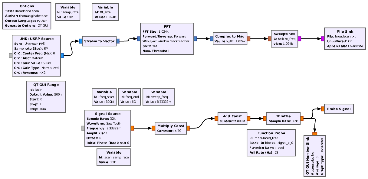
We need to read samples, measure the signal strength for a while, store it in a file, and also change frequency. Shouldn’t be too hard.

The missing pieces

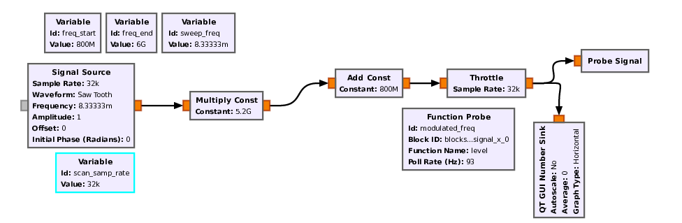
Automate changing frequency

We need to evenly increase the frequency, and when it reaches the top, go back to the beginning. That’s a saw tooth signal.

Then we need to stick that value into a variable. That’s what Probe Signal block is for.

So this part we can solve entirely with standard GNU Radio blocks.

Measure strength

The only piece I needed to write was a block that takes a frequency (from stream tags) and a stream of some float vectors (signal strength), and outputs frequency and signal strength.

It’s a very simple block. With not much code. It’s written for GNU Radio 3.8 and newer, but the changes are easy to backport to 3.7 for someone so inclined. The differences should just be in the yaml file that needs to be written in XML format instead.

Here’s the full flow graph:

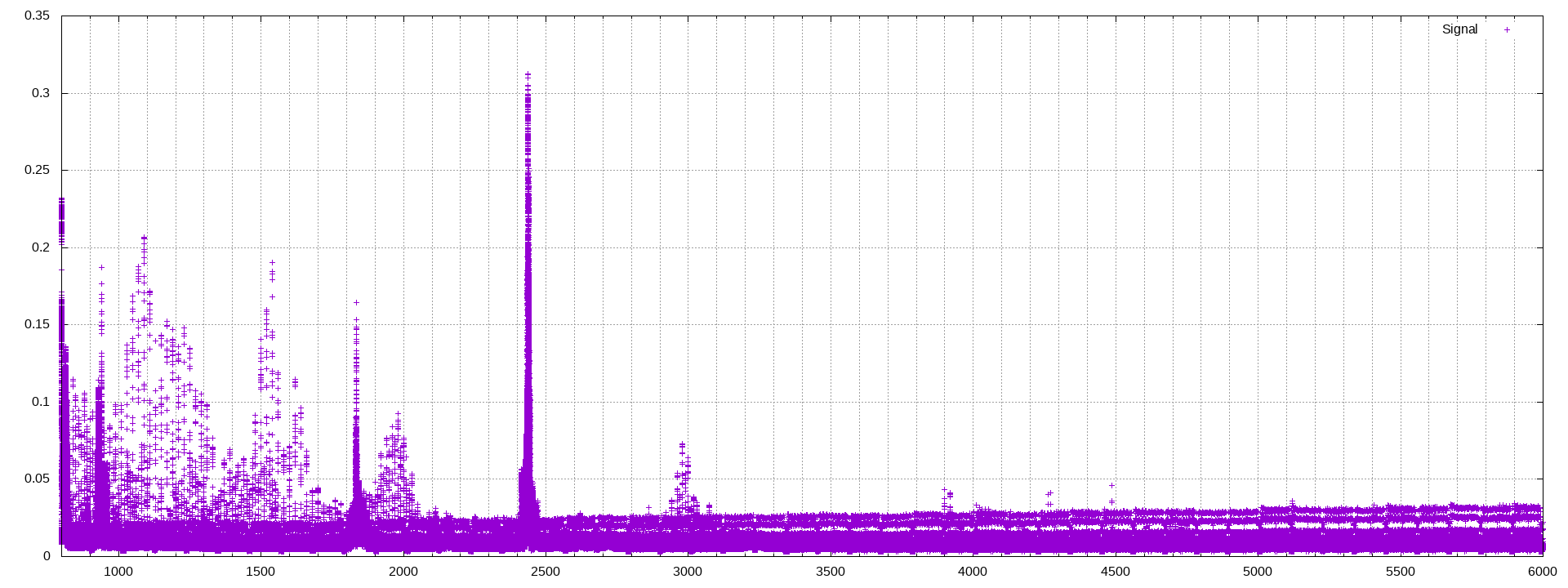
Results

The results can then be plotted by GNUPlot.

set terminal png truecolor rounded size 1920,720 enhanced
set output "broadband.png"
set xtics 500
set mxtics 5
set grid mxtics
set grid xtics
set grid ytics
plot [800:6000] "broadband-scan.txt" using ($2/1e6):3 with points title "Signal"

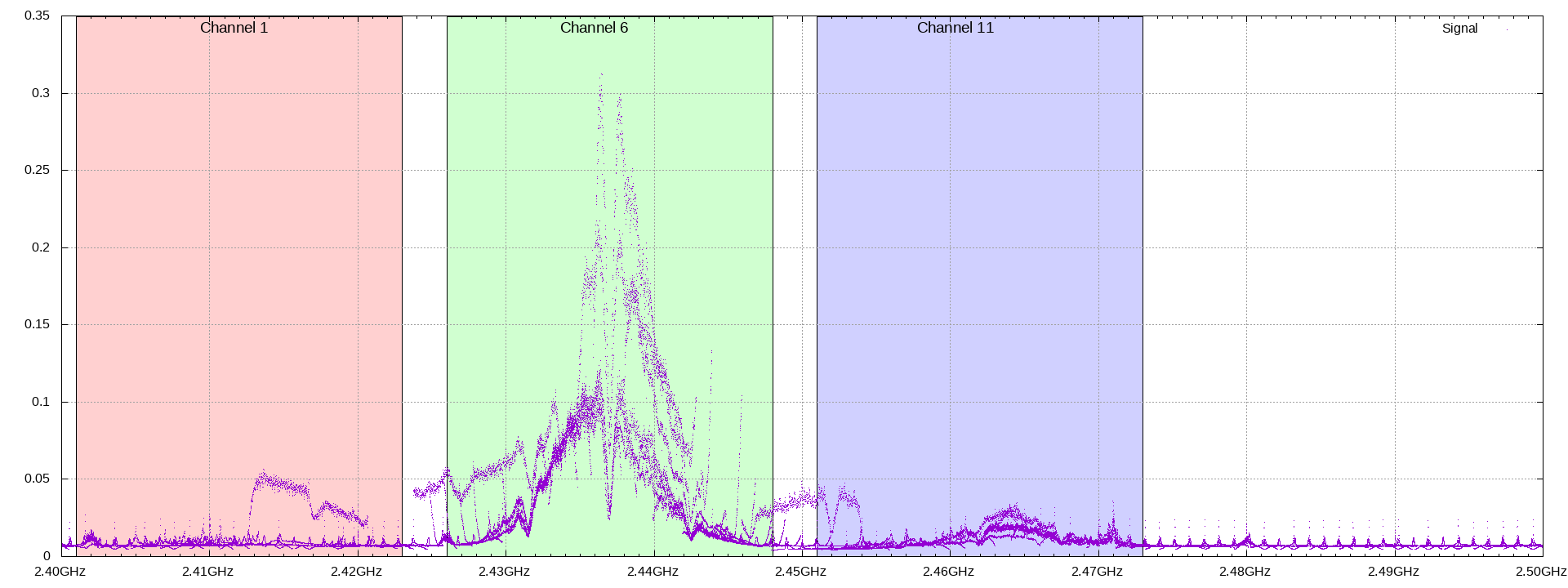
Or zoomed into 2.4GHz for a wifi survey:

set terminal png truecolor rounded size 1920,720 enhanced
set output "wifi.png"
set xtics 0.01
set mxtics 10
set grid xtics
set grid ytics
set object  1 rectangle from 2.401,0 to 2.423,100 fs solid fc rgb "#ffd0d0" behind
set object  6 rectangle from 2.426,0 to 2.448,100 fs solid fc rgb "#d0ffd0" behind
set object 11 rectangle from 2.451,0 to 2.473,100 fs solid fc rgb "#d0d0ff" behind
set format x "%.2fGHz"
set label  1 center at screen 0.15,0.95, char 1 "Channel 1"  font ",14"
set label  6 center at screen 0.38,0.95, char 1 "Channel 6"  font ",14"
set label 11 center at screen 0.61,0.95, char 1 "Channel 11" font ",14"
plot [2.4:2.5] "broadband-scan.txt" using ($2/1e9):3 with dots title "Signal"

Guess which wifi channel I’m using, when on 2.4GHz. :-)

Future work

This flow graph saves the timestamp of the measurements, but doesn’t use it. So this can also be used to analyze spectrum usage over time. And combined with a GPS logger this could be put on a car and plot the spectrum on a map, as well.

The antenna, and its big brother, is easily attached to a car window for such purposes.